Unit 3 · Topic 3.4 · about 30 minutes · 7 parts · 11 scored checks, 3 of them multiple choice, plus 2 from earlier lessons
AP Macroeconomics 3.4: Long-Run Aggregate Supply (LRAS)
Unit 3: 17 to 27% of the multiple-choice section
What you'll be able to do
- Define the short run and the long run, using a graph where it helps.
- Define the long-run aggregate supply (LRAS) curve, using a graph where it helps.
Key vocabulary
| Term | What it means | The exam trap |
|---|---|---|
| Short run | The period in which some input prices, such as wages set by contracts, are fixed and have not adjusted to a change in the price level. | Calendar time is not the test: the short run means some input prices, such as wages in a contract, are still fixed, however many months that lasts. |
| Long run | The period long enough for all prices and wages to be fully flexible and to adjust to the price level. | No trade-off between inflation and unemployment survives into the long run, so faster inflation does not buy lasting lower unemployment. |
| Long-run aggregate supply (LRAS) curve | The curve showing the real output an economy produces at each price level once wages and prices have fully adjusted, vertical at full-employment output. | Higher spending alone never moves LRAS; it shifts only when the economy's resources or technology change, so an AD shift leaves YF where it was. |
| Full-employment level of output | The real output an economy produces when unemployment equals its natural rate, labeled YF on an AD-AS graph. | Zero unemployment is not what YF means; at YF unemployment equals its natural rate, with frictional and structural unemployment still there. |
| Maximum sustainable capacity | The total output an economic system will produce over a set period of time if all resources are fully employed. | Sustainable is the word that matters: output can run past this level for a while with overtime and extra shifts, but it cannot stay there. |
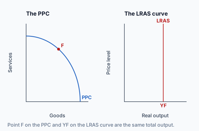
| Production possibilities curve (PPC) | A curve showing the combinations of two goods an economy can produce when all its resources are fully and efficiently employed. | Points inside the PPC match real output to the left of LRAS, and an outward PPC shift matches LRAS shifting right, not AD shifting right. |
 Tap to open the picture full size
Part 1 Think first Every price doubles
Guess before you learn. A wrong guess still makes the answer stick.
Predict first
Imagine every price in a country doubles. Store prices, hourly pay, rents, what firms pay for steel and fuel: all of it, twice what it was. The country has the same workers, the same factories and the same technology as before. Once everyone has adjusted to the new prices, how much real output does the country produce in a year?
In short. Long-run aggregate supply (LRAS) shows the real output an economy produces once every wage and price has adjusted, which is its full-employment level of output, YF.
- In the short run some input prices are fixed; in the long run all prices and wages are fully flexible.
- LRAS is a vertical line at full-employment output, labeled YF on the horizontal axis.
- LRAS and the production possibilities curve both show the economy's maximum sustainable capacity.
Part 2 Learn it Four short ideas, each checked as you go
2a. The short run and the long run
Economists split time by what has had a chance to adjust, not by a number of months.
In the short run, some input prices are fixed. A union contract sets wages for two years. A store's rent is locked by a lease. If the prices firms sell at rise while those costs stay put, each sale earns more, so firms hire and produce more. That is how output can run past its normal level for a while and unemployment can fall below its natural rate.
In the long run, all prices and wages are fully flexible. Contracts end and are rewritten, leases are renegotiated, and workers ask for pay that matches the higher prices. Once costs have caught up, the extra profit is gone, and so is the extra output.
One consequence matters for the rest of the course. In the short run, a burst of spending can bring lower unemployment along with higher inflation. In the long run there is no trade-off between the two: unemployment returns to its natural rate whatever the inflation rate turned out to be.
Quick check · Sort it
Tap a statement, then tap the time period it describes.
Short run
Long run
2b. Why LRAS is vertical
The long-run aggregate supply (LRAS) curve shows the real output the economy produces at each price level once all wages and prices have adjusted.
Try a price level 20 percent higher. In the long run, wages, rents and materials are all about 20 percent higher too. A firm that sells for 20 percent more but pays 20 percent more for everything it uses is no better off, so it has no reason to produce more. The same goes for a price level 20 percent lower. The numbers on the price tags change. The amount of real output does not.
So long-run output is set by the economy's resources and technology, used at full employment. That makes LRAS a vertical line at the full-employment level of output, labeled YF. Full employment is not zero unemployment. It means unemployment at its natural rate, with only frictional and structural unemployment left.
LRAS on the AD-AS graph
LRAS is vertical at full-employment output, YF. Here AD and SRAS cross on it.
Quick check · Decide and justify
An economy's price level rises 15 percent, and over the next few years every wage and input price rises 15 percent as well. In the long run, does the economy produce more real output than it did before the price level rose?
Which reason supports your choice?
2c. LRAS and the PPC
In Unit 1 you drew the production possibilities curve (PPC): the combinations of goods an economy can make when all its resources are fully employed. LRAS describes the same capacity. The PPC splits it between two goods; LRAS adds it up into one number, full-employment real output.
Both show the economy's maximum sustainable capacity: the total output it will produce over a set period, such as a year, if all its resources are fully employed. So the two graphs tell the same story:
- Production on the PPC is real output at LRAS, equal to YF.
- Production inside the PPC, with idle workers and machines, is real output to the left of LRAS.
- More resources or better technology push the PPC outward and shift LRAS to the right. Losing resources does the reverse.
Quick check · Match
Tap a situation, then tap what it means for the economy's PPC and its LRAS.
2d. Past YF, for a while
The word sustainable matters. YF is not the most an economy could ever squeeze out. For a time, firms can run extra shifts, put off maintenance, and hire people who would usually still be job hunting. Unemployment falls below its natural rate, and real output sits to the right of LRAS.
The economy cannot stay there. With jobs easy to find, workers win raises, and suppliers raise their prices. As input prices catch up, the extra output stops paying, and in the long run output returns to YF at a higher price level.
So LRAS marks the output the economy can keep up, not a wall it can never cross. That also means the economy does not move LRAS just by producing more: LRAS moves only when its resources or technology change.
Quick check · Multiple choice
Glenrock's real GDP this year is $830 billion. Economists estimate its full-employment output at $800 billion. Which statement best describes Glenrock's economy this year?
Part 3 Watch it done Wages catch up
Watch each step, then do the last one yourself.
A spending boom raises Brenmark's price level from 100 to 120. Its factory workers earn $25 an hour under contracts that cannot change for a year. Follow the real wage, and what it means for output, in the short run and in the long run.
Step 1 · The short run: the wage is stuck
For the year of the contracts, the nominal wage stays at $25. Deflated by the new price level, $25 ÷ 1.20 = $20.83, so the $25 now buys only what $20.83 bought before. Labor got cheaper in real terms while selling prices rose, so firms hire more and output rises above YF.
Why this step?
Why does a lower real wage lead firms to produce more?
Each hour of work now costs less compared with what that hour's output sells for, so hiring extra workers to make extra output pays. That is the short-run reason output can run past full employment.
Step 2 · The long run: contracts are rewritten
When the contracts end, workers bargain for pay that buys what $25 bought before prices rose. In the long run wages are fully flexible, so the new contracts deliver it.
Your step · Calculate
Finish the analysis. Brenmark's price level has risen from 100 to 120, and before the rise its factory workers earned $25 an hour. What nominal hourly wage, in dollars, leaves the real wage exactly where it was before the price level rose?
dollars
At $30 an hour, firms' costs have risen exactly as much as their prices, so the reason to produce extra output is gone and output returns to YF. Brenmark ends with a price level of 120 and the same long-run output it started with. The price level changed and long-run output did not, which is what a vertical LRAS says.
Part 4 Try it Watch where the long run lands
Try it · Multiple choice
Economies A and B have the same labor force, capital and technology. For many years aggregate demand in Economy A has been much higher than in Economy B at every price level, long enough for all wages and prices in both to adjust. Compared with Economy B, Economy A has
Part 5 Explain it Write it the way the exam asks
Nothing you type leaves this page.
Free response is 33.35% of the exam score. This one is shaped like Question 3, Short.
Free-response practice · Question 3 style
Assume the economy of Velmora is in long-run equilibrium. (a) Draw a correctly labeled graph of aggregate demand and aggregate supply showing the long-run aggregate supply curve at full-employment output labeled YF, the equilibrium price level labeled PL1 and real output labeled Y1. (b) Explain why the long-run aggregate supply curve is vertical. (c) Is Velmora producing at a point inside, on, or outside its production possibilities curve? Explain. (d) Suppose new technology raises how much Velmora's workers can produce in most industries. On your graph, show the effect on long-run aggregate supply, labeling the new curve LRAS2 and the new full-employment output YF2.
Model answer
(a) Price level on the vertical axis and real output on the horizontal, with a downward-sloping AD, an upward-sloping SRAS and a vertical LRAS at YF. AD and SRAS cross on LRAS at PL1 and Y1, so Y1 equals YF. (b) In the long run, wages and other input prices fully adjust to the price level, so a higher or lower price level leaves firms' real costs and profit per unit unchanged, and output stays at the full-employment level. (c) Velmora is producing on its PPC. In long-run equilibrium its output is at full employment, its maximum sustainable capacity, which is what a point on the PPC shows. (d) LRAS shifts right from the original LRAS to LRAS2, shown by an arrow, at YF2 to the right of YF.
Score your own answer. This is a self-check, not a grade. Tick each point your answer makes.
Part 6 Check yourself Read LRAS from real data
Read the table first, then answer the questions from it.
The U.S. Congressional Budget Office (CBO) estimates potential real GDP: the output the economy would produce with a high rate of use of its capital and labor. Economists use it as a measure of full-employment output, where LRAS sits. The table compares it with actual real GDP for three quarters, as FRED (Federal Reserve Bank of St. Louis) reported both series on October 14, 2026. CBO revises its estimates, so later readings can differ.
| Quarter | Actual real GDP | CBO potential real GDP |
|---|---|---|
| Q4 2018 | 20,305 | 20,294 |
| Q2 2020 | 19,078 | 20,926 |
| Q4 2023 | 23,033 | 22,678 |
Sources: U.S. Bureau of Economic Analysis, Real Gross Domestic Product (FRED series GDPC1), and U.S. Congressional Budget Office, Real Potential Gross Domestic Product (FRED series GDPPOT), both read October 14, 2026.
Case question 1 · Multiple choice
Treat CBO's potential real GDP as U.S. full-employment output. In Q2 2020, where was U.S. production compared with the U.S. PPC and LRAS?
Case question 2 · Calculate
Treat CBO's potential real GDP as U.S. full-employment output. Potential real GDP was 20,294 billion chained 2017 dollars in Q4 2018 and 22,678 billion in Q4 2023. By how many billions of chained 2017 dollars did U.S. LRAS shift to the right over those five years?
Case question 3 · Decide and justify
Treat CBO's potential real GDP as U.S. full-employment output. In Q4 2023, was potential real GDP, 22,678 billion chained 2017 dollars, the most the U.S. economy could produce that quarter?
Which reason supports your choice?
The rest stand on their own and do not use the case.
Check yourself · Fill the statement
Tap a blank, then tap a word or phrase.
The long-run aggregate supply curve is at the full-employment level of output, labeled on the horizontal axis, because in the long run wages and prices .
Check yourself · Spot the error
A student explained what happens after a spending boom pushes an economy's unemployment below its natural rate. Tap the first line that goes wrong.
Part 7 Keep it Keep it
From 3.3 Short-Run Aggregate Supply (SRAS) · Put it in order
In an economy, nominal wages are fixed by contracts and the labor force does not change. Tap the steps in the order they happen when the price level rises.
From 1.2 Opportunity Cost and the Production Possibilities Curve (PPC) · Select all
A country's PPC shifts outward. Which two statements must be true? Select two.
Select 2 answers, then check.
In three lines
- Short run: some input prices fixed. Long run: all wages and prices flexible.
- LRAS is vertical at full-employment output, YF, because wages and prices fully adjust.
- LRAS and the PPC both show maximum sustainable capacity, and they shift together.
Exam strategy for this topic
- Section I, Multiple Choice: 60 questions in 70 minutes.
- Section II, Free Response: 3 questions in 60 minutes.
- This lesson's Explain it is shaped like free-response question 3, Short.
- A four-function calculator is allowed on both sections of the exam.
Draw LRAS as a vertical line and label full-employment output YF where it meets the horizontal axis. When you explain why it is vertical, say that in the long run wages and prices fully adjust, so a different price level leaves real output unchanged.
Questions students ask
How long is the long run?
There is no set number of months. The long run is however long it takes for every wage and input price to adjust, which means contracts ending and leases being rewritten.
If the price level rises, why doesn't output rise in the long run?
Because costs rise with it. If the price level goes from 100 to 120, a worker paid $25 an hour will bargain up to $30, and a firm that sells for 20 percent more but pays 20 percent more for everything has no reason to produce more.
Can real GDP be bigger than full-employment output?
Yes, for a while. In the fourth quarter of 2023, U.S. real GDP was about 23,033 billion chained 2017 dollars against CBO's potential of 22,678 billion. Output past YF cannot last once wages and input prices catch up.
What shifts LRAS?
A change in the economy's resources or technology. A new power grid that lets every worker produce more shifts it right; skilled workers leaving the country for good shift it left.
How does LRAS connect to the PPC from Unit 1?
Both show maximum sustainable capacity. Producing on the PPC is output at LRAS, producing inside it is output to the left of LRAS, and when the PPC moves out, LRAS moves right.
Course alignment, for teachers
AP Macroeconomics topic 3.4, Unit 3: National Income and Price Determination.
- Skill 1.A: Describe economic concepts, principles, or models.
This lesson maps all 3 essential knowledge statements of the topic to the part that teaches each one: 3 are checked by a scored question. The map is in the lesson file.