Unit 3 · Topic 3.7 · about 30 minutes · 7 parts · 11 scored checks, 1 of them multiple choice, plus 2 from earlier lessons
AP Microeconomics 3.7: Perfect Competition
Unit 3: 22 to 25% of the multiple-choice section
What you'll be able to do
- Describe what makes a market perfectly competitive and efficient, explain with side-by-side graphs how a price-taking firm chooses its output and how prices move the market to an efficient long-run equilibrium, and calculate a firm's economic profit or loss from a graph or a table.
Key vocabulary
| Term | What it means | The exam trap |
|---|---|---|
| Perfectly competitive market | A market with many firms selling an identical product, where firms are free to enter and leave and no firm can affect the price. | Few real markets fit it exactly. It is a model, used as the benchmark other market structures are compared with. |
| Barriers to entry | Anything that keeps new firms from starting to sell in a market, such as a patent or a license limit. | Students sometimes count only government rules. A very large startup cost can keep new firms out just as well. |
| Market power | A firm's ability to raise its price without losing all of its customers. | Being large in sales is not the same thing; the test is whether the firm can change its price. |
| Price taker | A firm whose own output is too small a share of the market to change the market price, so it accepts that price. | The market price can still change when market demand or supply shifts. It is the single firm that cannot change it. |
| Marginal revenue (MR) | The extra revenue from selling one more unit. | Students divide total revenue by quantity and call it MR. That is average revenue, a different measure. |
| Marginal cost (MC) | The extra cost of producing one more unit. | It belongs to the last unit, not to every unit made; the average is a different curve. |
| Marginal benefit | The extra benefit a buyer gets from one more unit, shown by the height of the demand curve at that quantity. | Students mix it up with total benefit. It is about the last unit only. |
| Allocative efficiency | Producing the quantity at which the marginal benefit of the last unit equals its marginal cost. | It is about how much is made, not about whether each unit is cheap to make. |
| Productive efficiency | Producing output at the lowest possible average total cost. | Low marginal cost is not the test. Check which cost curve the definition names. |
| Efficient scale | The quantity of output at which a firm's average total cost is lowest. | Students look for it where MC bottoms out, which is at a smaller output. |
| Long-run equilibrium | A state in which every firm has adjusted all of its inputs and no firm wants to enter or leave the market. | A crossing of market demand and supply is not enough on its own; the firms must also have no reason to come or go. |
| Constant-cost industry | An industry whose firms' cost curves stay where they are as firms enter or leave. | Students mix up the firms' cost curves with the industry's long-run supply curve. They are on different graphs. |
| Increasing-cost industry | An industry whose firms' costs rise as the industry grows, often because entry bids up the price of an input it uses heavily. | Entry still happens when there is profit. What differs is where firms' costs end up once it has. |
| Decreasing-cost industry | An industry whose firms' costs fall as the industry grows, for example because a supplier can produce at a larger scale. | This is about the whole industry growing. Do not confuse it with one firm's economies of scale. |
 Tap to open the picture full size
Part 1 Think first The first taco trucks in town
Make a guess first. Even a wrong guess helps the answer stick.
Predict first
A city's first few taco trucks are packed every night, and their owners earn far more than they could in any other job. The city requires no special permit, and a used truck and kitchen gear are easy to buy. What do you expect to find five years later?
In short. In a perfectly competitive market, many price-taking firms each produce where price equals marginal cost, and this lesson follows such a market from the short run to the long run.
- The market's demand and supply set the price; each firm takes it as given, so for the firm P = MR, and it produces where P = MC.
- A firm's profit or loss in the short run comes from comparing the price with its ATC at the output it chooses.
- Where the long-run price ends after demand changes depends on whether the industry is constant cost, increasing cost or decreasing cost.
Part 2 Learn it Four ideas, with a check after each
2a. What makes a market perfectly competitive
A perfectly competitive market has many small firms selling an identical product, and nothing keeps new firms out: there are no barriers to entry. Many farm crops come close.
Each firm is a tiny share of the market, and its product is the same as everyone else's, so no firm has market power. Market demand and market supply set the price, and each firm takes it as given: it is a price taker.
- A firm can sell all the output it wants at that one price. Asking even a cent more sends its buyers to identical sellers, and asking less just gives revenue away.
- So the demand curve facing one firm is horizontal at the market price, and each extra unit sold adds exactly the price to revenue: P = MR.
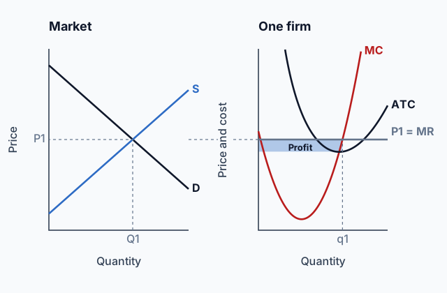
That is why perfect competition is drawn as two graphs side by side. The market graph, with its downward-sloping D and upward-sloping S, sets the price. The firm's graph carries that price across as a horizontal line labeled P = MR.
Quick check · Calculate
A wheat farm is one of thousands selling identical wheat, and the market price is $6 a bushel. The farm raises its output from 4,000 to 4,500 bushels, and nothing else in the market changes. By how many dollars does the farm's total revenue rise?
2b. The firm's choice, and the price as a signal
A price taker maximizes profit the way any firm does, at the output where MR = MC. Since its MR is the price, that is where P = MC, on the rising part of MC. On the firm's graph, read it where the horizontal price line meets MC.
The price also carries information in both directions:
- To buyers, it shows what the last unit cost a firm to make, because every firm produces up to where its marginal cost reaches the price.
- To firms, it shows what buyers will pay for one more unit, the marginal benefit of the last unit.
So at the market equilibrium, the price equals both the marginal benefit of the last unit consumed and the marginal cost of the last unit produced. MB = MC is allocative efficiency: every unit worth more to buyers than it costs to make gets made, and no unit that costs more than it is worth does.
The price also gives people a reason to act. If demand rises, the higher price tells firms that buyers value extra output above what it costs, and each firm moves up its MC curve to supply more.
Quick check · Calculate
In the perfectly competitive market for pecans, buyers want 9,000 pounds a week at $4 a pound, 8,000 at $5 and 7,000 at $6, and sellers offer 6,000 at $4, 8,000 at $5 and 10,000 at $6. One small farm grows pecans in 100-pound batches, and its marginal cost per pound is $3.00 for the 1st batch, $3.50 for the 2nd, $4.25 for the 3rd, $4.80 for the 4th, $5.40 for the 5th and $6.20 for the 6th. How many batches does the farm produce each week to maximize profit?
2c. From the short run to the long run
In a short-run equilibrium, the price can sit above or below its long-run level, so firms can earn profits or take losses.
- Price above minimum ATC: firms earn economic profit. New firms enter, market supply shifts right, and the price falls.
- Price below minimum ATC: firms take losses. Some leave, market supply shifts left, and the price rises.
Either way, the movement stops only when the price reaches the bottom of each firm's ATC. In that long-run equilibrium:
- P = MC, because each firm still produces where MR = MC;
- P = minimum ATC, so each firm earns zero economic profit, a normal profit, and produces at its efficient scale, the output with the lowest ATC.
On the firm's graph, the price line just touches the bottom of ATC, which is exactly where MC crosses ATC. On the market graph, the new supply curve crosses demand at that same price.
Quick check · Put it in order
The perfectly competitive market for kale is a constant-cost industry and starts in long-run equilibrium. Then demand for kale rises. Tap the events in the order they happen.
2d. Cost industries, and why the long run is efficient
Where the long-run price ends after a change in demand depends on what entry and exit do to firms' costs, and so on which part of the cost curves firms end up operating.
- Constant-cost industry: entry leaves each firm's cost curves where they were. After demand rises and firms enter, the price returns to the same minimum ATC. The long-run industry supply curve is horizontal.
- Increasing-cost industry: as the industry grows, entry bids up the price of inputs it uses heavily, such as specialized workers, so every firm's ATC shifts up. The long-run price ends higher than it began, and long-run supply slopes upward.
- Decreasing-cost industry: growth lowers firms' costs, for example when a supplier can reach a larger scale. The long-run price ends lower, and long-run supply slopes downward.
In each case, the long-run equilibrium is efficient in two senses. P = MC, so it is allocatively efficient. P = minimum ATC, so every firm produces at the lowest possible cost per unit and it is productively efficient.
Quick check · Sort it
Each card describes a perfectly competitive industry that started in long-run equilibrium. Tap a card, then tap the kind of industry it describes.
Constant cost
Increasing cost
Decreasing cost
Part 3 Watch it done From the market graph to one firm's loss
Follow each step, then finish the last one yourself.
The market for notebooks is perfectly competitive. Market demand is Qd = 90,000 − 5,000P and market supply is Qs = 10,000P − 30,000, with P in dollars and Q in notebooks a day. One typical firm's marginal cost is $6 at 300 notebooks a day, $8 at 400 and $10 at 500, and its ATC at those outputs is $10.00, $9.50 and $9.60. Find the market price, the firm's output, and its economic profit or loss.
Step 1 · Market price
Set quantity demanded equal to quantity supplied: 90,000 − 5,000P = 10,000P − 30,000, so 120,000 = 15,000P and P = $8. The market sells 90,000 − 40,000 = 50,000 notebooks a day.
Step 2 · The firm's output
The firm takes $8 as its MR and produces where MC = $8: 400 notebooks a day. The market's 50,000 notebooks come from 125 firms of this size.
Why this step?
Why does the firm use the market's $8 instead of looking at its own demand curve to choose a price?
It is a price taker. At any price above $8 its buyers go to identical sellers, and at $8 it can already sell all it wants, so its own demand is a horizontal line at $8, and $8 is its marginal revenue.
Step 3 · Profit per notebook
At 400 notebooks, ATC is $9.50, above the $8 price, so the firm loses 9.50 − 8 = $1.50 on each notebook.
Your step · Calculate
A firm in a perfectly competitive market sells notebooks at the market price of $8. It produces 400 notebooks a day, where its marginal cost is $8, and its average total cost there is $9.50. What is its economic profit, in dollars a day? Give a loss as a negative number.
dollars
Firms lose money at $8, so in the long run some leave. Market supply shifts left and the price rises until it reaches the bottom of the typical firm's ATC, where the loss is gone.
Part 4 Try it Draw the firm in four markets
Before each check, sketch the market graph on paper beside the lab: show which curve shifts and which way the price moves. Then say whether the firm earns a profit, a loss or zero economic profit at the new price.
Part 5 Explain it Answer a long free-response question
Nothing you type leaves this page. Draw the graphs on paper, then compare them with the model.
Free response is 33.35% of the exam score. This one is shaped like Question 1, Long.
Free-response practice · Question 1 style
The market for strawberries is perfectly competitive, is a constant-cost industry, and is in long-run equilibrium. (a) Draw correctly labeled side-by-side graphs for the strawberry market and for a typical strawberry farm. On the market graph, label the equilibrium price PE and quantity QE. On the farm's graph, show MC, ATC and the price, and label the farm's output qE. (b) What is the farm's economic profit? (c) Is the market allocatively efficient? Explain using price and marginal cost. (d) A study reports new health benefits of strawberries, and demand for them increases. On your market graph, show the new demand curve D2 and the new price P2. On the farm's graph, show P2 and label the farm's new output q2. (e) In the short run after the increase in demand, will the farm earn a positive, negative or zero economic profit? Explain. (f) In the long run, what happens to the number of farms in the market? Explain. (g) Compared with PE, will the new long-run price be higher, lower or the same? (h) In the new long-run equilibrium, is the typical farm productively efficient? Explain.
Model answer
(a) Market graph: price on the vertical axis, quantity on the horizontal, downward-sloping D1 and upward-sloping S crossing at PE and QE. Farm graph: price and cost on the vertical axis, quantity on the horizontal, MC rising through the lowest point of ATC, and a horizontal line at PE, labeled PE = MR, touching the bottom of ATC; qE is where MC meets that line. (b) Zero. The price equals ATC at qE. (c) Yes. Price equals marginal cost, so the marginal benefit buyers place on the last unit equals the cost of making it. (d) D2 to the right of D1, crossing S at a higher price P2 and a larger quantity. On the farm's graph, a higher horizontal line at P2, with q2 to the right of qE where it meets MC. (e) Positive. P2 is above ATC at q2. (f) The number of farms increases. Economic profit draws new farms in, and there are no barriers to entry. (g) The same. In a constant-cost industry, entry does not change farms' costs, so supply shifts right until the price is back at minimum ATC, PE. (h) Yes. The price equals minimum ATC, so each farm produces at the lowest possible average total cost.
The strawberry market
D1 and S cross at PE and QE. The increase in demand moves the curve to D2, which crosses S at the higher price P2 and the larger quantity Q2.
A typical strawberry farm
At PE the price line touches the bottom of ATC, where MC crosses it, so the farm makes qE and earns zero economic profit. At P2 it moves up MC to q2, where the price is above ATC.
Score your own answer. This is a self-check, not a grade. Tick each point your answer makes.
Part 6 Check yourself Basil: the market and one farm
The case questions can all be answered from the graph and the table.
Fresh basil is sold in a perfectly competitive market, and anyone may start a basil farm. The graph shows the whole market, where the price is set. The table beside it shows the daily total cost of Green Row, one typical basil farm, which takes that price as given. Green Row's fixed cost is $17 a day.
The market for basil
Market demand D and market supply S cross at a price of $12 a crate and a quantity of 400 thousand crates a day.
| Crates a day | Total cost |
|---|---|
| 0 | $17 |
| 1 | $26 |
| 2 | $32 |
| 3 | $36 |
| 4 | $42 |
| 5 | $50 |
| 6 | $61 |
| 7 | $75 |
| 8 | $94 |
Case question 1 · Calculate
At the market price, what is Green Row's economic profit at its profit-maximizing output, in dollars a day?
Case question 2 · Decide and justify
If every basil farm has costs like Green Row's, what will happen to the number of basil farms in the long run?
Which reason supports your choice?
Case question 3 · Multiple choice
Suppose Green Row's costs are typical and basil farms' costs do not change as farms enter or leave. What will the market price of a crate be once the market reaches long-run equilibrium?
The rest stand on their own and do not use the case.
Check yourself · Select all
A perfectly competitive market is in long-run equilibrium. Which two statements are true? Select two.
Select 2 answers, then check.
Check yourself · Spot the error
Demand for oat milk rises in a perfectly competitive market, and the market price climbs from $3 to $4 a carton. Firms' costs do not change. A student explained what happens next. Tap the first line with a mistake.
Check yourself · Rank it
Three perfectly competitive industries start in long-run equilibrium. Industry A is a constant-cost industry, Industry B an increasing-cost industry and Industry C a decreasing-cost industry. In each, market demand increases by the same amount at every price, and firms enter until a new long-run equilibrium is reached. Rank the industries by how much market quantity rises from the old long-run equilibrium to the new one.
Largest increase first
Give each one a place, 1 for first. Give two the same place if they are equal.
Your ranking: none yet
Part 7 Keep it Keep it
From 3.6 Firms’ Short-Run Decisions to Produce and Long-Run Decisions to Enter or Exit a Market · Calculate
A firm in a perfectly competitive market has a fixed cost of $40. Its total variable cost is $30 for 1 unit, $50 for 2 units, $66 for 3 units, $92 for 4 units and $130 for 5 units. What is the lowest price, in dollars, at which the firm will produce rather than shut down in the short run?
From 3.4 Types of Profit · Sort it
Jonah quit his job as a mechanic to open a bike-repair shop. He paid for its tools partly with his own savings and partly with a bank loan. Tap each item, then tap the kind of cost it is for the shop.
Explicit cost
Implicit cost
In three lines
- A price taker faces a horizontal demand at the market price, so P = MR, and it produces where P = MC.
- Short-run profit draws firms in and losses push them out, until P = MC = minimum ATC and economic profit is zero.
- That long-run equilibrium is allocatively and productively efficient, and the long-run price depends on whether costs stay the same, rise or fall as the industry grows.
Exam strategy for this topic
- Section I, Multiple Choice: 60 questions in 70 minutes.
- Section II, Free Response: 3 questions in 60 minutes.
- This lesson's Explain it is shaped like free-response question 1, Long.
- A four-function calculator is allowed on both sections of the exam.
Draw perfect competition as two graphs side by side, with the price levels lined up: the market's D and S set the price, and a dashed line carries it across to the firm, where it is the horizontal P = MR. Label the firm's quantity where MR = MC. For long-run equilibrium, draw that line touching the bottom of ATC, where MC crosses it.
Questions students ask
Why is the firm's demand curve horizontal when the market's slopes down?
One firm is a tiny share of the market. It can sell all it wants at the market price and nothing above it, so the demand it faces is flat at that price, even though buyers in the market as a whole buy less when the price rises.
If firms earn zero economic profit in the long run, why do they stay?
Zero economic profit is a normal profit. Revenue covers every cost, including what the owners could have earned elsewhere, so they do as well here as in their next-best choice and have no reason to leave.
What is the difference between allocative and productive efficiency?
Allocative efficiency is about how much is made: P = MC, so the last unit's value to buyers equals its cost. Productive efficiency is about how it is made: at the lowest possible ATC. Perfect competition in long-run equilibrium achieves both.
How do I calculate a firm's profit from a graph?
Find the quantity where MR = MC. At that quantity, subtract ATC from the price to get profit per unit, then multiply by the quantity. A price below ATC gives a negative number, a loss.
Does the long-run price always return to where it started?
Only in a constant-cost industry. In an increasing-cost industry growth raises firms' costs, so the price ends higher; in a decreasing-cost industry it ends lower.
Course alignment, for teachers
AP Microeconomics topic 3.7, Unit 3: Production, Cost, and the Perfect Competition Model.
- Skill 4.A: Draw an accurately labeled graph or visual to represent an economic model or market.
This lesson maps all 9 essential knowledge statements of the topic to the part that teaches each one: 9 are checked by a scored question. The map is in the lesson file.