Unit 3 · Topic 3.3 · about 30 minutes · 7 parts · 12 scored checks, 2 of them multiple choice, plus 2 from earlier lessons

AP Microeconomics 3.3: Long-Run Production Costs

Built by Tanner Crow from College Board's course framework · Every answer key independently checked

Unit 3: 22 to 25% of the multiple-choice section

What you'll be able to do

Define returns to scale and economies and diseconomies of scale, explain with a long-run average total cost curve how cost per unit changes as a whole firm grows and how minimum efficient scale shapes a market, and calculate long-run average total cost from a table.

Key vocabulary

Term	What it means	The exam trap
Long run	A period long enough for a firm to change all of its inputs, including its plant and equipment.	How long the long run lasts depends on the industry: a food truck can change its size in weeks, while a steel mill takes years.
Variable cost	A cost that changes with the quantity the firm produces.	A variable cost can be known in advance. What makes it variable is that it rises or falls with the quantity produced.
Scale of production	The size of a firm's whole operation, measured by the quantities of all its inputs together.	Adding workers to the same plant does not change the scale; scale changes when the plant changes too.
Increasing returns to scale	Output rises by a larger percentage than all the inputs rise together.	It is a long-run idea. In the short run, with some input fixed, use marginal product instead.
Constant returns to scale	Output rises by the same percentage as all the inputs rise together.	Constant describes how output responds to scale. It does not mean the firm's output stays constant.
Decreasing returns to scale	Output rises by a smaller percentage than all the inputs rise together.	Students mix it up with diminishing marginal returns, which come from adding one input to fixed ones in the short run.
Long-run average total cost (LRATC)	The lowest average total cost of producing each output when the firm can choose the plant size that suits that output best.	It is not the ATC curve of any one plant. Each point may use a different plant size.
Economies of scale	A range of output over which LRATC falls as the firm grows.	Economies of scale describe one range of output, not the firm at every size, so check which range a question asks about.
Diseconomies of scale	A range of output over which LRATC rises as the firm grows.	They come from the firm's own size, such as the difficulty of managing a huge operation, not from a rise in input prices.
Efficient scale	The range of output over which LRATC is at its lowest level.	Efficient here is about cost per unit, not about whether the firm makes the goods buyers value most.
Minimum efficient scale (MES)	The smallest output at which LRATC reaches its lowest level.	MES is a quantity of output, not a cost.
Market concentration	How much of a market's sales are made by its largest few firms.	High concentration says the largest few firms make most of the sales. On its own it does not tell you their prices.
Market structure	The kind of market a good is sold in, described by features such as the number of firms and how easily new firms can enter.	Market structure describes the whole market, not one firm's plans.

Three short-run average total cost curves, SRATC1, SRATC2 and SRATC3, for a small, a medium and a large plant, with output on the horizontal axis and cost per unit on the vertical axis. Each curve is U-shaped and sits further right than the one before. The medium plant's lowest point is lower than the small plant's, and the large plant's lowest point is higher than the medium plant's.

Part 1 Think first Jets and haircuts

Make a guess first. Even a wrong guess helps the answer stick.

Predict first

In a large country, a few companies build almost all of the passenger jets, while tens of thousands of separate businesses cut hair. Which do you think best explains the difference?

In short. In the long run a firm can change the size of its whole operation, and its long-run average total cost falls, stays flat or rises as it grows.

Returns to scale compare the percentage rise in output with the percentage rise in all inputs: increasing, constant or decreasing.
Falling LRATC is economies of scale, the flat stretch is constant returns to scale (the efficient scale), and rising LRATC is diseconomies of scale.
Minimum efficient scale, the smallest output with the lowest LRATC, helps decide how many firms a market can hold.

Part 2 Learn it Four ideas, with a check after each

2a. In the long run, every cost is variable

In the long run a firm can change every input. It can sign a new lease, build a second plant, sell machines or close a store. So in the long run all costs are variable. There is no total fixed cost and no AFC.

That changes the question the firm asks. In the short run it asks how many workers to add to the plant it has. In the long run it asks what size of plant to have at all.

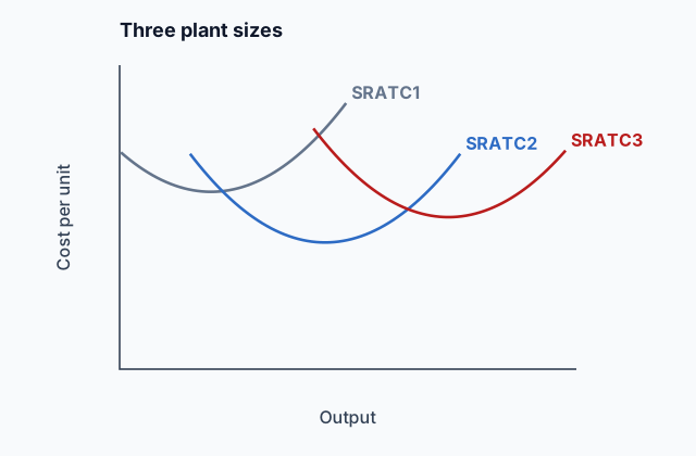
Each plant size has its own short-run ATC curve, like the three in the picture near the top of this page. The long-run average total cost (LRATC) curve shows the lowest average total cost of producing each output when the firm can pick whichever plant size suits that output best.

A lease shows the difference. This year the rent is fixed, because the lease cannot be undone. In a plan for the next ten years it is variable: the firm can renew the lease, move or take more space.

Quick check · Multiple choice

A bakery pays $3,000 a month in rent under a lease that ends in two years. It is planning how big to be over the next ten years, long enough to change all of its inputs. In that plan, how should the bakery treat the rent?

2b. Returns to scale

Returns to scale describe what happens to output when a firm changes all of its inputs by the same percentage, which it can do only in the long run.

Increasing returns to scale: output rises by a larger percentage than the inputs. Double every input and output more than doubles.
Constant returns to scale: output rises by the same percentage. Double every input and output doubles.
Decreasing returns to scale: output rises by a smaller percentage. Double every input and output rises, but less than double.

Compare percentages, not amounts. A bakery that goes from 10 workers and 2 ovens to 20 workers and 4 ovens has raised every input by 100%. If its output goes from 500 to 1,200 loaves a day, a rise of 140%, it has increasing returns to scale.

Keep this apart from diminishing marginal returns in 3.1 The Production Function. That was one input added to fixed ones in the short run. Returns to scale change every input together, so nothing is fixed.

Quick check · Sort it

Each card describes a firm that changes all of its inputs by the same percentage. Tap a card, then tap the returns to scale it shows.

Increasing returns to scale

Constant returns to scale

Decreasing returns to scale

2c. The shape of long-run average total cost

Returns to scale show up in cost per unit. If output grows faster than the inputs while input prices stay the same, each unit costs less. So the LRATC curve has up to three stretches.

Economies of scale: LRATC falls as output rises. A bigger firm can split work into narrower jobs and use large, specialized machines that a small firm could not keep busy.
Constant returns to scale: LRATC is flat as output rises. This flat stretch at the lowest cost per unit is called the efficient scale.
Diseconomies of scale: LRATC rises as output rises. A very large firm is hard to run: instructions pass through more layers of managers, and departments get harder to coordinate.

To read the stretches from a table, compare LRATC at each output with LRATC at the output before it. Falling means economies of scale, unchanged means constant returns, and rising means diseconomies.

Quick check · Decide and justify

A firm's long-run average total cost is $12 a unit at 1,000 units a week, $9 at 2,000, $8 at 3,000, $8 at 4,000, $8 at 5,000 and $10 at 6,000. Which describes the firm as it grows from 3,000 to 5,000 units a week?

Which reason supports your choice?

2d. Minimum efficient scale and the number of firms

Minimum efficient scale (MES) is the smallest output at which LRATC reaches its lowest level, where economies of scale run out. A firm smaller than that has a higher cost per unit than a rival producing anywhere on the flat stretch of LRATC.

Compare MES with the quantity buyers want at a price equal to that lowest LRATC.

If MES is small next to that quantity, many firms can each reach the lowest cost. Expect many firms and low market concentration, as with hair salons.
If MES is large next to it, the market has room for only a few firms of efficient size, so expect a few large firms and high concentration. If MES is about as big as the whole market, one firm can supply it at the lowest cost.

A quick estimate of the number of firms: divide the quantity buyers want by MES. If buyers want 900,000 units and MES is 300,000, at most 3 firms can each produce at MES. That is how cost helps set a market structure, the subject of the rest of the course.

Quick check · Calculate

In a market for bricks, buyers want 600,000 tons a year at a price equal to the lowest long-run average total cost. A brick maker's LRATC first reaches that lowest level at 150,000 tons a year and stays there up to 300,000 tons. What is the largest number of brick makers that could each produce at least the minimum efficient scale?

Your answer firms

Common mistakes

The mistake	Why it is wrong	Do this instead
Treating rent or another cost as fixed in the long run.	In the long run the firm can change every input, so every cost can change.	Say all costs are variable in the long run, and leave fixed cost and AFC out of long-run analysis.
Mixing up diminishing marginal returns with decreasing returns to scale.	Diminishing marginal returns come from adding one input to fixed ones in the short run; returns to scale change every input together.	Use returns to scale only when every input changes by the same percentage.
Taking minimum efficient scale to be the largest output at the lowest cost.	MES is where LRATC first reaches its lowest level, where economies of scale end.	Find the first output at which LRATC hits its minimum.

Part 3 Watch it done How big should a chair maker be?

Follow each step, then finish the last one yourself.

A furniture maker can build a plant of any size. Its long-run total cost is $20,000 a week at 1,000 chairs, $32,000 at 2,000, $42,000 at 3,000, $56,000 at 4,000, $70,000 at 5,000 and $90,000 at 6,000. Find its LRATC at each output, the ranges of economies of scale, constant returns to scale and diseconomies of scale, and its minimum efficient scale.

Step 1 · LRATC
Divide each total by its output. LRATC is $20, $16, $14, $14, $14 and $15 a chair at 1,000 to 6,000 chairs.
Step 2 · The three ranges
LRATC falls from 1,000 to 3,000 chairs: economies of scale. It stays at $14 from 3,000 to 5,000: constant returns to scale. It rises past 5,000: diseconomies of scale.
Why this step?
Why might the cost per chair rise once the maker goes past 5,000 chairs a week, when it can choose every input freely?
A very large operation is harder to manage. Instructions pass through more layers and departments are harder to coordinate, so each chair takes more management cost even with the best plant for that output.
Your step · Calculate

A furniture maker's long-run average total cost is $20 a chair at 1,000 chairs a week, $16 at 2,000, $14 at 3,000, $14 at 4,000, $14 at 5,000 and $15 at 6,000. What is its minimum efficient scale, in chairs a week?

Your answer chairs

Part 4 Try it Draw the long-run average total cost curve

Work out each point first. Divide each long-run total cost by its output. Before you sketch, name the range of output where the cement maker has economies of scale.

Try it · Sketch the graph

A cement maker can choose any plant size. Its long-run total cost is $40,000 a month at 2,000 tons, $45,000 at 3,000 tons, $60,000 at 4,000 tons, $75,000 at 5,000 tons and $102,000 at 6,000 tons. Sketch its long-run average total cost at each of these outputs. The first point is fixed at $20 a ton for 2,000 tons.

Drag a point up or down, or tap it and use the arrow keys. Only the shape is checked.

Part 5 Explain it Answer a short free-response question

Nothing you type leaves this page. Draw the graph on paper, then compare it with the model.

Free response is 33.35% of the exam score. This one is shaped like Question 3, Short.

Free-response practice · Question 3 style

Northfield Glass makes windows and can change all of its inputs in the long run. (a) Draw a correctly labeled graph of Northfield's long-run average total cost (LRATC) curve that shows economies of scale, constant returns to scale and diseconomies of scale. Label the minimum efficient scale QMES. (b) Northfield doubles every input it uses, and its output rises by 50%. Identify whether Northfield has increasing, constant or decreasing returns to scale. (c) Suppose the minimum efficient scale in the window industry is large compared with the quantity of windows buyers want. Will the industry tend to have many small firms or a few large firms? Explain.

Your answer stays on this page. It is never sent or saved.

Model answer

(a) Cost per unit on the vertical axis and output on the horizontal axis. LRATC falls (economies of scale), then is flat (constant returns to scale), then rises (diseconomies of scale). QMES is the output where the flat stretch begins, the smallest output at which LRATC reaches its lowest level. (b) Decreasing returns to scale: output rose by 50%, a smaller percentage than the 100% rise in inputs. (c) A few large firms. Only a firm producing at least the minimum efficient scale reaches the lowest cost per unit, and when that output is large next to what buyers want, the market has room for only a few such firms. Smaller firms would have higher costs per unit and be undersold.

Long-run average total cost

LRATC falls (economies of scale), is flat (constant returns to scale) and then rises (diseconomies of scale). QMES marks the smallest output at which LRATC is lowest.

Score your own answer. This is a self-check, not a grade. Tick each point your answer makes.

(a) Correctly labeled axes and an LRATC curve that falls, then is flat, then rises.
(a) QMES is labeled at the output where LRATC first reaches its lowest level.
(b) Identifies decreasing returns to scale.
(c) Says the industry tends to have a few large firms.
(c) Explains that only firms at or beyond the large minimum efficient scale reach the lowest cost per unit, and the market has room for only a few of them.

Part 6 Check yourself Four industries in Norland

The case questions can all be answered from this table.

Norland is a large country. For four of its industries, the table shows the minimum efficient scale of one firm and the quantity buyers in Norland want each year at a price equal to the industry's lowest long-run average total cost.

Minimum efficient scale and market quantity in Norland each year
Industry	Minimum efficient scale of one firm	Quantity buyers want
Cement	2,000,000 tons	6,000,000 tons
Haircuts	4,000 haircuts	8,000,000 haircuts
Breakfast cereal	50,000 tons	400,000 tons
Passenger jets	600 jets	900 jets

Case question 1 · Calculate

What is the largest number of cement firms in Norland that could each produce at least the minimum efficient scale?

Your answer firms

Case question 2 · Multiple choice

Which of the four industries in Norland is most likely to be dominated by one or two large firms?

Case question 3 · Rank it

Rank three of Norland's industries by the largest number of firms that could each produce at least the minimum efficient scale.

Most firms first

Give each one a place, 1 for first. Give two the same place if they are equal.

Cement
Haircuts
Breakfast cereal

Your ranking: none yet

The rest stand on their own and do not use the case.

Check yourself · Spot the error

A firm raises its workers from 20 to 40 and its machines from 5 to 10, and its output rises from 1,000 to 1,800 units a week. A student classified its returns to scale. Tap the first line with a mistake.

Check yourself · Select all

A firm's long-run average total cost falls as it grows from 1,000 to 3,000 units a week. Which two statements about that range are correct? Select two.

Select 2 answers, then check.

Check yourself · Fill the statement

Tap a blank, then tap a word or phrase.

A restaurant chain plans for the long run, when it can change every input. In that plan its total fixed cost is , and the rent on each of its buildings is a cost.

Part 7 Keep it Keep it

From 3.2 Short-Run Production Costs · Match

A firm's total fixed cost is $40. At 4 units of output its total variable cost is $80, and at 3 units its total cost was $105. Tap a measure, then tap its value at 4 units.

From 2.5 Other Elasticities · Calculate

When a household's income rises from $40,000 to $60,000 a year, with prices unchanged, its restaurant meals rise from 10 to 14 a month. Using the midpoint method, what is its income elasticity of demand for restaurant meals? Round to two decimal places, and give a negative number if it is negative.

Your answer

In three lines

In the long run a firm can change every input, so all of its costs are variable.
Returns to scale compare the percentage change in output with the percentage change in all inputs; LRATC falls with economies of scale, is flat with constant returns and rises with diseconomies.
Minimum efficient scale is the smallest output with the lowest LRATC, and a large MES next to market demand means few firms.

Exam strategy for this topic

Section I, Multiple Choice: 60 questions in 70 minutes.
Section II, Free Response: 3 questions in 60 minutes.
This lesson's Explain it is shaped like free-response question 3, Short.
A four-function calculator is allowed on both sections of the exam.

When you draw LRATC, show it falling, then flat, then rising, and label each stretch: economies of scale, constant returns to scale, diseconomies of scale. Label minimum efficient scale where the flat stretch begins. For returns to scale, compare percentage changes, and say plainly that every input changed.

Questions students ask

What is the difference between decreasing returns to scale and diminishing marginal returns?

Diminishing marginal returns are short run: one input is added to fixed ones, and each addition adds less output. Decreasing returns to scale are long run: every input grows by the same percentage, and output grows by a smaller percentage.

Why are there no fixed costs in the long run?

A cost is fixed only because some input cannot be changed yet. In the long run every lease can end and every machine can be bought or sold, so every cost can change.

Why does LRATC eventually rise?

A very large firm is hard to manage. Information passes through more layers, and coordinating many plants and departments costs more, so cost per unit climbs even with the best plant for each output.

Does every industry have a U-shaped LRATC?

No. Some have a long flat stretch, and in some the cost per unit keeps falling across the whole range buyers want. The shape, and where MES falls, differ from industry to industry.

How does minimum efficient scale affect the number of firms?

Divide the quantity buyers want by MES. A small result means only a few firms can reach the lowest cost, so the market tends to be concentrated; a large result leaves room for many.

Course alignment, for teachers

AP Microeconomics topic 3.3, Unit 3: Production, Cost, and the Perfect Competition Model.

Skill 1.D: Describe the similarities, differences, and limitations of economic concepts, principles, or models.

This lesson maps all 4 essential knowledge statements of the topic to the part that teaches each one: 4 are checked by a scored question. The map is in the lesson file.