Unit 2 · Topic 2.15 · about 30 minutes · 7 parts · 14 scored checks, 2 of them multiple choice

Semi-log Plots

Built from College Board's course framework · Every answer key independently checked

A semi-log plot with a base 10 y-axis: the marks 1, 10, 100, 1,000 and 10,000 are evenly spaced, with unevenly spaced minor marks between them, and the x-axis is an ordinary scale from 0 to 10. The exponential data y = 3(2)^x, from 3 at x = 0 to 3,072 at x = 10, lie on a straight line. The linear data y = 300x + 50, from 50 to 3,050, bend downward on the same axes.

Part 1 Think first

New graph paper

Guess before you learn. A wrong guess still makes the answer stick.

Predict first

A lab technician counts a bacteria culture every hour: 3, 6, 12 and 24 thousand cells, and so on, up to 3,072 thousand at hour 10. On ordinary graph paper the first seven points are squashed flat against the bottom. She switches to paper whose y-axis is marked 1, 10, 100, 1000 and 10,000, with those marks evenly spaced. What shape do the eleven points make on the new paper?

In short. A semi-log plot scales its y-axis logarithmically, so data that grow or decay exponentially show up as a straight line.

With base 10, the y-axis marks 1, 10, 100 and 1000 are evenly spaced, and a value $y$ sits at height $\log y$ .
If the logarithms of the outputs trend linear for large inputs, a transformation of an exponential function fits the data, with no need to subtract a constant first.
For $y = a b^{x}$ the line on the plot is $\log_{n} y = (\log_{n} b) x + \log_{n} a$ . Undo the slope to get $b$ and the intercept to get $a$ .

Part 2 Learn it

Four short ideas, each checked as you go

2a. A y-axis that counts factors

On ordinary graph paper, equal steps up the y-axis add the same amount: 0, 100, 200, 300. On a semi-log plot, one axis is logarithmically scaled instead, with some base $n > 1$ . Here that is always the y-axis. The x-axis stays an ordinary number line.

With base 10, the y-axis marks read 1, 10, 100, 1000, evenly spaced, and each step up multiplies by 10. A value $y$ is placed at height $\log y$ , so 100 sits two steps up. The minor marks for 2, 3, and so on up to 9 times a power of 10 are placed at their logarithms too, which is why they crowd toward the top of each step. A base 2 axis works the same way, with marks 1, 2, 4, 8, 16.

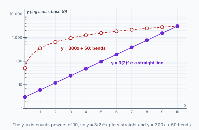
Now look at the diagram. For $y = 3 (2)^{x}$ , each step of 1 in $x$ multiplies $y$ by 2, so every point climbs the same distance, $\log 2 \approx 0.301$ of a step. Equal climbs make a straight line. When the y-axis is logarithmically scaled, data that show exponential characteristics appear linear. Decay does too: $y = 800 (0.5)^{x}$ drops the same distance each step, a line sloping down.

The linear data $y = 300 x + 50$ add 300 each time. That is a large factor at 50 and a small one at 2750, so the points bend.

Quick check · Sort it

No calculator. Each card lists the outputs of a data set at $x = 0, 1, 2$ and $3$ . Tap a card, then say how its points look on a semi-log plot with a base 10 y-axis.

On a straight line

Not on a straight line

2b. When the logs trend linear

Real data are rarely a clean $a b^{x}$ . Here is a data set where you do not know the formula. Take the base 10 logarithm of each output. Those are the heights of the points on a semi-log plot.

A data set and the base 10 logarithms of its outputs
$x$	$y$	$\log y$	Change in $\log y$
0	52	1.716
1	56	1.748	0.032
2	68	1.833	0.085
3	104	2.017	0.184
4	212	2.326	0.309
5	536	2.729	0.403
6	1508	3.178	0.449
7	4424	3.646	0.468
8	13172	4.120	0.474

The changes start small, grow, and settle near 0.47. On the semi-log plot the points curve at first and then run along a line.

That is the test. If, for large input values, the logarithms of the outputs trend linear, then a transformation of an exponential function can model the data. (These outputs are $2 (3)^{x} + 50$ . The 50 matters while $2 (3)^{x}$ is small and hardly at all once it is in the thousands.)

Notice what you skipped. In 2.5 Exponential Function Context and Data Modeling you subtracted a constant, such as the room temperature, before the ratios came out equal. A semi-log plot reveals the exponential trend without transforming the outputs by a constant first.

Quick check · Decide and justify

No calculator. A data set has positive outputs. For the inputs $x = 0, 1, 2, \dots, 9$ , the base 10 logarithms of its outputs are 2.310, 2.326, 2.373, 2.489, 2.719, 3.069, 3.494, 3.952, 4.422 and 4.897. Which kind of model do these logarithms support?

Which reason supports your answer?

2c. Line tools on a log axis

Once the points on a semi-log plot lie along a line, every tool you have for lines works on it: slope from two points, the intercept, point-slope form. Just remember what the vertical coordinate is. It is $\log y$ , not $y$ .

Say two points on a base 10 semi-log line are labeled $(2, 30)$ and $(6, 3000)$ , as $(x, y)$ . Their heights are $\log 30$ and $\log 3000$ . From 30 to 3000 is a factor of 100, which is two powers of 10, so the rise is 2. The run is 4.

slope = \frac{\log 3000 - \log 30}{6 - 2} = \frac{2}{4} = 0.5

So $\log y$ goes up 0.5 for each 1 in $x$ . Every 2 units of $x$ add 1 to $\log y$ , which multiplies $y$ by 10. The intercept works the same way: it is the height $\log y$ where $x = 0$ .

The slip is to use the printed labels as if the axis were ordinary. $\frac{3000 - 30}{4} = 742.5$ is a slope on ordinary graph paper and means nothing here. Take the logarithm of each value first, then subtract.

Quick check · Calculate

No calculator. Two points on a line drawn on a semi-log plot with a base 10 y-axis are labeled $(1, 4)$ and $(5, 4000)$ , as $(x, y)$ . What is the slope of the line in the plot's own units, the change in $\log y$ for each increase of 1 in $x$ ?

Your answer

2d. Back to the exponential model

Here is why exponential data line up. Take the logarithm, base $n$ , of both sides of $y = a b^{x}$ and use the product and power properties:

\log_{n} y = (\log_{n} b) x + \log_{n} a

With $\log_{n} y$ as the vertical coordinate, that is a line. Its rate of change is $\log_{n} b$ and its initial value is $\log_{n} a$ . This is the linearization of the exponential data.

To get back to the exponential model, undo the logarithm on each number, using the plot's base. Suppose a base 10 semi-log line is $\log y = 0.5 x + 1.2$ . Then $\log b = 0.5$ , so $b = 10^{0.5} \approx 3.16$ . And $\log a = 1.2$ , so $a = 10^{1.2} \approx 15.8$ . The model is $y \approx 15.8 (3.16)^{x}$ .

If the plot were base 2 instead, the same line would give $b = 2^{0.5} \approx 1.41$ and $a = 2^{1.2}$ . The base of the axis is the base you undo with.

A falling line has a negative slope, and $10$ to a negative power is between 0 and 1. So a falling semi-log line means $0 < b < 1$ , which is decay.

Quick check · Spot the error

No calculator. A student turns a semi-log line back into an exponential model. Tap the line where the mistake is first made.

Part 3 Watch it done

From counts to a model

Watch each step, then do the last one yourself.

A biology class counts yeast cells in a sample, in thousands per milliliter, every 2 hours. At $t = 0, 2, 4, 6$ and $8$ hours the counts are 12, 30, 75, 188 and 469. Use a semi-log plot with a base 10 y-axis to decide whether an exponential model fits, then find the model $y = a b^{t}$ .

Step 1 · Take the logarithms
The heights on the semi-log plot are $\log 12 \approx 1.079$ , $\log 30 \approx 1.477$ , $\log 75 \approx 1.875$ , $\log 188 \approx 2.274$ and $\log 469 \approx 2.671$ .
Step 2 · Look for a line
The changes in height are 0.398, 0.398, 0.399 and 0.397 for each 2 hours. Equal changes mean the points lie on a line, so an exponential model fits.
Step 3 · Slope and intercept
Use the first and last points. The slope is $\frac{2.671 - 1.079}{8 - 0} = 0.199$ per hour, and the height at $t = 0$ is 1.079. The linear model for the plot is $\log y = 0.199 t + 1.079$ .
Why this step?
Why is the intercept 1.079 equal to $\log a$ rather than $a$ ?
Because the vertical coordinate on the plot is $\log y$ . At $t = 0$ the model gives $y = a b^{0} = a$ , so that point sits at height $\log a$ .
Step 4 · Undo the intercept
$\log a = 1.079$ , so $a = 10^{1.079} \approx 12.0$ thousand cells per milliliter.
Your step · Calculate

Graphing calculator required. Finish it. The slope of the semi-log line is 0.199 per hour, and it equals $\log b$ . What is $b$ ? Give three decimal places.

Your answer

Part 4 Try it

A line that falls

In this invented example, a nurse records the amount of a medicine in a patient's blood, in milligrams, every hour after a dose. On a semi-log plot with a base 10 y-axis, the readings lie close to a line through the points $(0, 400)$ and $(6, 100)$ , where $t$ is hours after the dose. Every example so far has climbed. This one falls.

Try it · Decide and justify

No calculator. On the nurse's semi-log plot, the readings fall on a line from $(0, 400)$ to $(6, 100)$ , with $t$ in hours. Which model fits them?

Which reason supports your answer?

Try it · Calculate

Graphing calculator required. Use the two points on the nurse's semi-log line, $(0, 400)$ and $(6, 100)$ , to find $b$ in the model $y = 400 b^{t}$ . Give three decimal places.

Your answer

Part 5 Explain it

Write it the way the exam asks

Nothing you type leaves this page.

Free response is 37.5% of the exam score. This one is shaped like Question 2, Modeling a Non-Periodic Context.

Free-response practice · Question 2 style

Graphing calculator required. Algae are spreading across a pond. A biologist measures the covered area $A$ , in square meters, every 3 days. At $d = 0, 3, 6, 9$ and $12$ days the areas are 2.0, 5.4, 14.6, 39.4 and 106.3, and their base 10 logarithms are 0.301, 0.732, 1.164, 1.595 and 2.027. (i) Explain why an exponential model is appropriate for these data, using a semi-log plot with a base 10 y-axis. (ii) Using the logarithms at $d = 0$ and $d = 12$ , write the linear model $\log A = m d + k$ for the semi-log plot. (iii) Write an exponential model $A = a b^{d}$ for the data. (iv) Use your model to estimate the covered area at $d = 15$ .

Your answer stays on this page. It is never sent or saved.

Model answer

(i) On a semi-log plot the points sit at heights 0.301, 0.732, 1.164, 1.595 and 2.027. These rise by 0.431 or 0.432 every 3 days, so the points lie on a line. Data that appear linear on a semi-log plot can be modeled by an exponential function. (ii) $m = \frac{2.027 - 0.301}{12 - 0} \approx 0.1438$ and $k = 0.301$ , so $\log A = 0.1438 d + 0.301$ . (iii) $b = 10^{0.1438} \approx 1.393$ and $a = 10^{0.301} \approx 2.000$ , so $A = 2.000 (1.393)^{d}$ . (iv) $A = 2.000 (1.393)^{15} \approx 289$ square meters.

Score your own answer. This is a self-check, not a grade. Tick each point your answer makes.

Explains that the logarithms rise by equal amounts, so the points are linear on the semi-log plot and an exponential model is appropriate.
Writes $\log A = 0.1438 d + 0.301$ , with the slope found from the two logarithms.
Writes $A = 2.000 (1.393)^{d}$ by undoing both the slope and the intercept with base 10.
Estimates an area of about 287 to 289 square meters at $d = 15$ , using the model.

Part 6 Check yourself

One table of scooter counts

The two case questions use the same table. Answer them from it.

A city counts the electric scooters $N$ available to rent $w$ weeks after a rental program started. The table gives $N$ and its base 10 logarithm, rounded to three decimal places.

Scooters available, $N$ , after $w$ weeks
$w$	$N$	$\log N$
0	46	1.663
1	52	1.716
2	64	1.806
3	88	1.944
4	136	2.134
5	232	2.365
6	424	2.627
7	808	2.907
8	1576	3.198

Case question 1 · Multiple choice

No calculator. The points $(w, N)$ for the scooter counts are plotted on a semi-log plot with a base 10 y-axis. Which describes the plotted points?

Case question 2 · Calculate

Graphing calculator required. Use the values of $\log N$ at $w = 6$ and $w = 8$ in the scooter table to find the slope of the semi-log trend line for large $w$ . That slope equals $\log b$ . What is the weekly growth factor $b$ ? Give two decimal places.

Your answer

The rest stand on their own and do not use the case.

Check yourself · Match

No calculator. Each equation is the linear model for a semi-log plot with a base 10 y-axis, where the vertical coordinate is $\log y$ . Tap an equation, then the exponential model it comes from.

Check yourself · Fill the statement

No calculator. On a semi-log plot with a base 10 y-axis, data lie along a line with slope 0.3. Tap a blank, then tap an answer.

Each time $x$ increases by 1, the height $\log y$ goes up by . Each time $x$ increases by 10, $y$ is multiplied by .

Check yourself · Select all

No calculator. Which two statements about a semi-log plot with a base 10 y-axis are true? Pick two.

Select 2 answers, then check.

Part 7 Keep it

Bring back earlier ideas

Pulling an older idea back up is what makes it last.

From 2.9 Logarithmic Expressions · Multiple choice

No calculator. On a base 10 logarithmic scale, point P is 3 units to the right of point Q. How does the number at P compare with the number at Q?

From 2.5 Exponential Function Context and Data Modeling · Decide and justify

No calculator. Tea is poured at 90 degrees Celsius in a 20 degree room. Every 5 minutes it reads 90, 76, 64.8 and 55.84 degrees. Which model fits, with $t$ in minutes?

Which reason supports your answer?

In three lines

A semi-log plot scales the y-axis logarithmically with base $n > 1$ , so exponential data appear linear.
If the logarithms of the outputs trend linear for large inputs, a transformed exponential function fits, with no constant to subtract first.
For $y = a b^{x}$ the line is $\log_{n} y = (\log_{n} b) x + \log_{n} a$ : slope $\log_{n} b$ , initial value $\log_{n} a$ , each undone with base $n$ .

Unit 2 check: 15 questions from every lesson in Unit 2

Vocabulary

Semi-log plot: A graph in which one axis, here always the y-axis, is logarithmically scaled with base $n$ , where $n > 1$ .
Logarithmically scaled axis: An axis on which a value $y$ is placed at height $\log_{n} y$ , so the marks 1, $n$ , $n^{2}$ , $n^{3}$ are evenly spaced.
Linearization: Rewriting exponential data $y = a b^{x}$ as the line $y = (\log_{n} b) x + \log_{n} a$ on a semi-log plot, where the vertical coordinate is the logarithm of the output.
Linear rate of change: The slope of the semi-log line, $\log_{n} b$ , from which the base $b$ of the exponential model is recovered.
Initial linear value: The height of the semi-log line at input 0, $\log_{n} a$ , from which the initial value $a$ of the exponential model is recovered.

Course alignment, for teachers

AP Precalculus topic 2.15, Unit 2: Exponential and Logarithmic Functions.

Skill 2.B: Construct equivalent graphical, numerical, analytical, and verbal representations of functions that are useful in a given mathematical or applied context, with and without technology.
Skill 3.C: Support conclusions or choices with a logical rationale or appropriate data.

This lesson maps all 4 essential knowledge statements of the topic to the part that teaches each one: 4 are checked by a scored question. The map is in the lesson file.